Simple Sales Prediction
01_intro
02_conversion
03_averages
04_difference
05_product
06_sum
07_the_omegas
08_coefficients
09_prediction
10_visualized
11_reduction
12_to_wide
99_appendix
One Page
Intro
You have a years worth of sales data for 2 shops, for 6 products. Use simple linear regression to predict the sales for the next month. Tool to use: Apache Spark dataframes.
You receive the data in this 'wide' format, and beware: not all of the cells have data! Spot the 'nulls'.
scala> sale_df.orderBy("shop","product").show()

|----------+-------+----+----+----+----+----+----+----+----+----+----+----+----+
|      shop|product| jan| feb| mar| apr| may| jun| jul| aug| sep| oct| nov| dec|
|----------+-------+----+----+----+----+----+----+----+----+----+----+----+----+
|  megamart|  bread| 371| 432| 425| 524| 468| 414|null| 487| 493| 517| 473| 470|
|  megamart| cheese|  51|  56|  63|null|  66|  66|  50|  56|  58|null|  48|  50|
|  megamart|   milk|null|  29|  26|  30|  26|  29|  29|  25|  27|null|  28|  30|
|  megamart|   nuts|1342|1264|1317|1425|1326|1187|1478|1367|1274|1380|1584|1156|
|  megamart| razors| 599|null| 500| 423| 574| 403| 609| 520| 495| 577| 491| 524|
|  megamart|   soap|null|   7|   8|   9|   9|   8|   9|   9|   9|   6|   6|   8|
|superstore|  bread| 341| 398| 427| 344| 472| 370| 354| 406|null| 407| 465| 402|
|superstore| cheese|  57|  52|null|  54|  62|null|  56|  66|  46|  63|  55|  53|
|superstore|   milk|  33|null|null|  33|  30|  36|  35|  34|  38|  32|  35|  29|
|superstore|   nuts|1338|1369|1157|1305|1532|1231|1466|1148|1298|1059|1216|1231|
|superstore| razors| 360| 362| 366| 352| 365| 361| 361| 353| 317| 335| 290| 406|
|superstore|   soap|   8|   8|   7|   8|   6|null|   7|   7|   7|   8|   6|null|
|----------+-------+----+----+----+----+----+----+----+----+----+----+----+----+
(in the appendix of this article, you'll find the Scala code that creates this dataframe)
All the data manipulation is done in Spark Dataframes.
These dataframe functions are used:
groupBy(..).agg( sum(..), avg(..) )withColumn()withColumnRenamed()join()drop()select(), ..
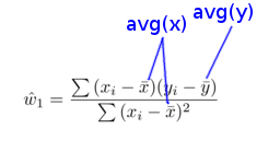
Formula
Here's the formula to calculate the coefficients for the simple linear regression, picked up from article Simple Linear Regression :

From wide to narrow
To make it easier to do the calculations, first we convert the dataframe from wide to narrow, so that we end up with this format:
         shop   product   unit   month
 ------------ --------- ------ -------
   superstore     bread    341       1
   superstore    cheese     57       1
   superstore    razors    360       1
   superstore      soap      8       1
   superstore      milk     33       1
   superstore      nuts   1338       1
     megamart     bread    371       1
     megamart    cheese     51       1
     megamart    razors    599       1
           ..
           ..
The naive, elaborate way of doing the conversion from wide to narrow would be to create 12 dataframes like this, and unionall them together:
     val d1=sale_df.select("shop","product","jan").
                    withColumnRenamed("jan","unit").
                    withColumn("month", lit(1) )

     val d2=sale_df.select("shop","product","feb").
                    withColumnRenamed("feb","unit").
                    withColumn("month", lit(2) )
     ..
     ..
     val d12=sale_df.select("shop","product","dec").
                    withColumnRenamed("dec","unit").
                    withColumn("month", lit(12) )

     df=d1.unionAll(d2).unionAll(d3).unionAll(d4). .. unionAll(d12)
But there is an easier way: do it programmatically, as shown in the following bit of Scala code. This is a lot more elegant, and saves a lot of typing (and typos) :
    val months=Seq("jan","feb","mar","apr","may","jun","jul","aug","sep","oct","nov","dec")

    var i=0
    val df_seq = for (  m <- months ) yield {
                        i=i+1
                        sale_df.select("shop","product",m).
                            withColumnRenamed(m,"unit").
                            withColumn("month", lit(i) )
                    }
    val df=df_seq.reduce( _ unionAll _ )
The resulting dataframe looks like this:
df.orderBy("shop","product","month").show()

+--------+-------+----+-----+
|    shop|product|unit|month|
+--------+-------+----+-----+
|megamart|  bread| 371|    1|
|megamart|  bread| 432|    2|
|megamart|  bread| 425|    3|
|megamart|  bread| 524|    4|
|megamart|  bread| 468|    5|
|megamart|  bread| 414|    6|
|megamart|  bread|null|    7|
|megamart|  bread| 487|    8|
|megamart|  bread| 493|    9|
|megamart|  bread| 517|   10|
|megamart|  bread| 473|   11|
|megamart|  bread| 470|   12|
|megamart| cheese|  51|    1|
|megamart| cheese|  56|    2|
|megamart| cheese|  63|    3|
|megamart| cheese|null|    4|
..
..
To make it easier on our brain to grok the mathematical formula, let's rename the 'unit' column to 'y' and the 'month' column to 'x', like used in the above formula. At the same time, let's already filter out the records where the unit is null, they are of no use to the calculations.
    val sale_narrow_df=df.where("unit is not null").
                          withColumnRenamed("unit","y").
                          withColumnRenamed("month","x").
                          select("shop","product","x","y")
Narrow dataframe: sale_narrow_df
Completing the conversion from wide to narrow, we end up with this dataframe, on which all the following calculations will be based.
sale_narrow_df.orderBy("shop","product","x").show()

+--------+-------+---+---+
|    shop|product|  x|  y|
+--------+-------+---+---+
|megamart|  bread|  1|371|
|megamart|  bread|  2|432|
|megamart|  bread|  3|425|
|megamart|  bread|  4|524|
|megamart|  bread|  5|468|
|megamart|  bread|  6|414|
|megamart|  bread|  8|487|
|megamart|  bread|  9|493|
|megamart|  bread| 10|517|
|megamart|  bread| 11|473|
|megamart|  bread| 12|470|
|megamart| cheese|  1| 51|
|megamart| cheese|  2| 56|
|megamart| cheese|  3| 63|
|megamart| cheese|  5| 66|
|megamart| cheese|  6| 66|
..
..Calculate the averages: groupBy(..).agg(avg(..))
Let's kick off the calculations, first we do the averages of x and y:
val a1 = sale_narrow_df.groupBy("shop","product").agg( avg("x"), avg("y") )Result:
a1.orderBy("shop","product").show()

+----------+-------+------------------+------------------+
|      shop|product|            avg(x)|            avg(y)|
+----------+-------+------------------+------------------+
|  megamart|  bread| 6.454545454545454|461.27272727272725|
|  megamart| cheese|               6.4|              56.4|
|  megamart|   milk|               6.7|              27.9|
|  megamart|   nuts|               6.5|1341.6666666666667|
|  megamart| razors| 6.909090909090909| 519.5454545454545|
|  megamart|   soap|               7.0|               8.0|
|superstore|  bread|6.2727272727272725|398.72727272727275|
|superstore| cheese|               6.9|              56.4|
|superstore|   milk|               7.3|              33.5|
|superstore|   nuts|               6.5|1279.1666666666667|
|superstore| razors|               6.5| 352.3333333333333|
|superstore|   soap|               6.0|               7.2|
+----------+-------+------------------+------------------+
Naming convention
When short name chosen for a dataframe starts with an 'a' (eg a1,a2,...) it's about an aggregate (ie at shop/product level), and when it starts with a 'd' (eg. d1,d2,..) it's about a detail (ie. at the lowest level: shop/product/month~unit)
Cosmetics
For the sake of this document: let's round off the above averages to retain just 4 digits after the decimal point, just to be able to fit more columns of data onto 1 row! When concerned with precision, please skip this step.
User defined rounding function:
def udfRound = udf[Double,Double] { (x) => Math.floor( x*10000.0 + 0.5 )/10000.0 } Round off:
    val a2=a1.withColumn("avg_x", udfRound( a1("avg(x)") )).
              withColumn("avg_y", udfRound( a1("avg(y)") )).
              select("shop","product","avg_x","avg_y")
Result:
a2.orderBy("shop","product").show()

+----------+-------+------+---------+
|      shop|product| avg_x|    avg_y|
+----------+-------+------+---------+
|  megamart|  bread|6.4545| 461.2727|
|  megamart| cheese|   6.4|     56.4|
|  megamart|   milk|   6.7|     27.9|
|  megamart|   nuts|   6.5|1341.6666|
|  megamart| razors| 6.909| 519.5454|
|  megamart|   soap|   7.0|      8.0|
|superstore|  bread|6.2727| 398.7272|
|superstore| cheese|   6.9|     56.4|
|superstore|   milk|   7.3|     33.5|
|superstore|   nuts|   6.5|1279.1666|
|superstore| razors|   6.5| 352.3333|
|superstore|   soap|   6.0|      7.2|
+----------+-------+------+---------+
'Glue' these averages onto dataframe sale_narrow_df, using a left-outer join :
val d1= sale_narrow_df.join( a2, Seq("shop","product"), "leftouter")Result:
d1.orderBy("shop","product","x").show()

+--------+-------+---+---+------+--------+
|    shop|product|  x|  y| avg_x|   avg_y|
+--------+-------+---+---+------+--------+
|megamart|  bread|  1|371|6.4545|461.2727|
|megamart|  bread|  2|432|6.4545|461.2727|
|megamart|  bread|  3|425|6.4545|461.2727|
|megamart|  bread|  4|524|6.4545|461.2727|
|megamart|  bread|  5|468|6.4545|461.2727|
|megamart|  bread|  6|414|6.4545|461.2727|
|megamart|  bread|  8|487|6.4545|461.2727|
|megamart|  bread|  9|493|6.4545|461.2727|
|megamart|  bread| 10|517|6.4545|461.2727|
|megamart|  bread| 11|473|6.4545|461.2727|
|megamart|  bread| 12|470|6.4545|461.2727|
|megamart| cheese|  1| 51|   6.4|    56.4|
|megamart| cheese|  2| 56|   6.4|    56.4|
|megamart| cheese|  3| 63|   6.4|    56.4|
..
..Difference between each element and the average of all elements
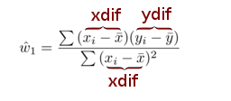
Calculate the dif between the x-values and avg(x), and the same for the y-values and avg(y) :
    val d2=d1.withColumn("xd", col("x")-col("avg_x")).
              withColumn("yd", col("y")-col("avg_y"))

    // apply cosmetics: round off
    val d3=d2.withColumn("xdif", udfRound( d2("xd") )).
              withColumn("ydif", udfRound( d2("yd") )).
              drop("xd").drop("yd")
Result:
d3.orderBy("shop","product","x").show()

+--------+-------+---+---+------+--------+-------+--------+
|    shop|product|  x|  y| avg_x|   avg_y|   xdif|    ydif|
+--------+-------+---+---+------+--------+-------+--------+
|megamart|  bread|  1|371|6.4545|461.2727|-5.4545|-90.2727|
|megamart|  bread|  2|432|6.4545|461.2727|-4.4545|-29.2727|
|megamart|  bread|  3|425|6.4545|461.2727|-3.4545|-36.2727|
|megamart|  bread|  4|524|6.4545|461.2727|-2.4546| 62.7273|
|megamart|  bread|  5|468|6.4545|461.2727|-1.4546|  6.7273|
|megamart|  bread|  6|414|6.4545|461.2727|-0.4546|-47.2727|
|megamart|  bread|  8|487|6.4545|461.2727| 1.5454| 25.7273|
|megamart|  bread|  9|493|6.4545|461.2727| 2.5454| 31.7273|
|megamart|  bread| 10|517|6.4545|461.2727| 3.5455| 55.7273|
|megamart|  bread| 11|473|6.4545|461.2727| 4.5455| 11.7273|
|megamart|  bread| 12|470|6.4545|461.2727| 5.5455|  8.7273|
|megamart| cheese|  1| 51|   6.4|    56.4|   -5.4|    -5.4|
|megamart| cheese|  2| 56|   6.4|    56.4|   -4.4|    -0.4|
|megamart| cheese|  3| 63|   6.4|    56.4|   -3.4|     6.6|
|megamart| cheese|  5| 66|   6.4|    56.4|-1.4001|     9.6|
|megamart| cheese|  6| 66|   6.4|    56.4|-0.4001|     9.6|
|megamart| cheese|  7| 50|   6.4|    56.4| 0.5999|    -6.4|
|megamart| cheese|  8| 56|   6.4|    56.4| 1.5999|    -0.4|
|megamart| cheese|  9| 58|   6.4|    56.4| 2.5999|     1.6|
|megamart| cheese| 11| 48|   6.4|    56.4|    4.6|    -8.4|
+--------+-------+---+---+------+--------+-------+--------+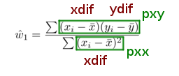
    val d4=d3.withColumn("p_xy", col("xdif")*col("ydif") ).
              withColumn("p_xx", col("xdif")*col("xdif") )

    // apply cosmetics: round off
    val d5=d4.withColumn("pxy", udfRound( d4("p_xy") )).
              withColumn("pxx", udfRound( d4("p_xx") )).
              drop("p_xy").
              drop("p_xx")
Result:
d5.orderBy("shop","product","x").show()

+--------+-------+---+---+------+--------+-------+--------+---------+-------+
|    shop|product|  x|  y| avg_x|   avg_y|   xdif|    ydif|      pxy|    pxx|
+--------+-------+---+---+------+--------+-------+--------+---------+-------+
|megamart|  bread|  1|371|6.4545|461.2727|-5.4545|-90.2727| 492.3924|29.7515|
|megamart|  bread|  2|432|6.4545|461.2727|-4.4545|-29.2727| 130.3952|19.8425|
|megamart|  bread|  3|425|6.4545|461.2727|-3.4545|-36.2727|  125.304|11.9335|
|megamart|  bread|  4|524|6.4545|461.2727|-2.4546| 62.7273|-153.9705|  6.025|
|megamart|  bread|  5|468|6.4545|461.2727|-1.4546|  6.7273|  -9.7856| 2.1158|
|megamart|  bread|  6|414|6.4545|461.2727|-0.4546|-47.2727|  21.4901| 0.2066|
|megamart|  bread|  8|487|6.4545|461.2727| 1.5454| 25.7273|  39.7589| 2.3882|
|megamart|  bread|  9|493|6.4545|461.2727| 2.5454| 31.7273|  80.7586|  6.479|
|megamart|  bread| 10|517|6.4545|461.2727| 3.5455| 55.7273| 197.5811|12.5705|
|megamart|  bread| 11|473|6.4545|461.2727| 4.5455| 11.7273|  53.3064|20.6615|
|megamart|  bread| 12|470|6.4545|461.2727| 5.5455|  8.7273|  48.3972|30.7525|
|megamart| cheese|  1| 51|   6.4|    56.4|   -5.4|    -5.4|    29.16|  29.16|
|megamart| cheese|  2| 56|   6.4|    56.4|   -4.4|    -0.4|     1.76|  19.36|
|megamart| cheese|  3| 63|   6.4|    56.4|   -3.4|     6.6|   -22.44|11.5599|
|megamart| cheese|  5| 66|   6.4|    56.4|-1.4001|     9.6|  -13.441| 1.9602|
|megamart| cheese|  6| 66|   6.4|    56.4|-0.4001|     9.6|   -3.841|   0.16|
|megamart| cheese|  7| 50|   6.4|    56.4| 0.5999|    -6.4|  -3.8394| 0.3598|
|megamart| cheese|  8| 56|   6.4|    56.4| 1.5999|    -0.4|    -0.64| 2.5596|
|megamart| cheese|  9| 58|   6.4|    56.4| 2.5999|     1.6|   4.1598| 6.7594|
|megamart| cheese| 11| 48|   6.4|    56.4|    4.6|    -8.4|   -38.64|21.1599|
+--------+-------+---+---+------+--------+-------+--------+---------+-------+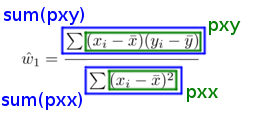
val a3=d5.groupBy("shop","product").agg( sum("pxy"), sum("pxx") )Result:
a3.orderBy("shop","product").show()

+----------+-------+-------------------+------------------+
|      shop|product|           sum(pxy)|          sum(pxx)|
+----------+-------+-------------------+------------------+
|  megamart|  bread| 1025.6277999999998|142.72660000000002|
|  megamart| cheese|           -83.6016|124.39869999999998|
|  megamart|   milk|  4.699600000000002|          100.0994|
|  megamart|   nuts|  466.9998999999999|             143.0|
|  megamart| razors|           -69.4553|120.90820000000001|
|  megamart|   soap|              -11.0|             110.0|
|superstore|  bread|           596.8173|136.18159999999997|
|superstore| cheese|0.39890000000000114|          128.8991|
|superstore|   milk|-2.5002999999999993|          104.0996|
|superstore|   nuts|         -2096.0004|             143.0|
|superstore| razors|-285.00030000000004|             143.0|
|superstore|   soap|           -11.0003|             110.0|
+----------+-------+-------------------+------------------+Divide to get ω₁
val a4=a3.withColumn("w1", col("sum(pxy)")/col("sum(pxx)") )Result:
a4.orderBy("shop","product").show()

+----------+-------+-------------------+------------------+--------------------+
|      shop|product|           sum(pxy)|          sum(pxx)|                  w1|
+----------+-------+-------------------+------------------+--------------------+
|  megamart|  bread| 1025.6277999999998|142.72660000000002|   7.185961131281762|
|  megamart| cheese|           -83.6016|124.39869999999998| -0.6720456081936549|
|  megamart|   milk|  4.699600000000002|          100.0994|0.046949332363630567|
|  megamart|   nuts|  466.9998999999999|             143.0|   3.265733566433566|
|  megamart| razors|           -69.4553|120.90820000000001| -0.5744465635912204|
|  megamart|   soap|              -11.0|             110.0|                -0.1|
|superstore|  bread|           596.8173|136.18159999999997|   4.382510559429469|
|superstore| cheese|0.39890000000000114|          128.8991|0.003094668620649...|
|superstore|   milk|-2.5002999999999993|          104.0996|-0.02401834397058...|
|superstore|   nuts|         -2096.0004|             143.0| -14.657345454545453|
|superstore| razors|-285.00030000000004|             143.0| -1.9930090909090912|
|superstore|   soap|           -11.0003|             110.0|-0.10000272727272727|
+----------+-------+-------------------+------------------+--------------------+
Calculate ω₀
Glue column ω₁ onto aggregation dataframe a2 (which has the averages), so that we can compute ω₀ from the formula:

    val a5= a2.join( a4, Seq("shop","product"), "leftouter").
               select("shop","product","avg_x","avg_y","w1")
Result:
a5.orderBy("shop","product").show()

+----------+-------+------+---------+--------------------+
|      shop|product| avg_x|    avg_y|                  w1|
+----------+-------+------+---------+--------------------+
|  megamart|  bread|6.4545| 461.2727|   7.185961131281762|
|  megamart| cheese|   6.4|     56.4| -0.6720456081936549|
|  megamart|   milk|   6.7|     27.9|0.046949332363630567|
|  megamart|   nuts|   6.5|1341.6666|   3.265733566433566|
|  megamart| razors| 6.909| 519.5454| -0.5744465635912204|
|  megamart|   soap|   7.0|      8.0|                -0.1|
|superstore|  bread|6.2727| 398.7272|   4.382510559429469|
|superstore| cheese|   6.9|     56.4|0.003094668620649...|
|superstore|   milk|   7.3|     33.5|-0.02401834397058...|
|superstore|   nuts|   6.5|1279.1666| -14.657345454545453|
|superstore| razors|   6.5| 352.3333| -1.9930090909090912|
|superstore|   soap|   6.0|      7.2|-0.10000272727272727|
+----------+-------+------+---------+--------------------+
Now calculate w0:
val a6=a5.withColumn("w0", col("avg_y") - col("w1") * col("avg_x") ) Result:
a6.orderBy("shop","product").show()

+----------+-------+------+---------+--------------------+------------------+
|      shop|product| avg_x|    avg_y|                  w1|                w0|
+----------+-------+------+---------+--------------------+------------------+
|  megamart|  bread|6.4545| 461.2727|   7.185967535361064|  414.890872543012|
|  megamart| cheese|   6.4|     56.4| -0.6720257234726688| 60.70096463022508|
|  megamart|   milk|   6.7|     27.9| 0.04695304695304696|27.585414585414583|
|  megamart|   nuts|   6.5|1341.6667|   3.265738461538462|         1320.4394|
|  megamart| razors|6.9091| 519.5455| -0.5744354248425476| 523.5143317937795|
|  megamart|   soap|   7.0|      8.0|                -0.1|               8.7|
|superstore|  bread|6.2727| 398.7273|   4.382494922243877| 371.2372241012408|
|superstore| cheese|   6.9|     56.4|0.003103180760279...| 56.37858805275407|
|superstore|   milk|   7.3|     33.5|-0.02401536983669545| 33.67531219980788|
|superstore|   nuts|   6.5|1279.1667| -14.657339160839161|1374.4394045454546|
|superstore| razors|   6.5| 352.3333| -1.9930055944055944|365.28783636363636|
|superstore|   soap|   6.0|      7.2|                -0.1| 7.800000000000001|
+----------+-------+------+---------+--------------------+------------------+ val coeff_df= a6.select("shop","product","w0","w1").cache()Here the final result:
coeff_df.orderBy("shop","product").show()

+----------+-------+------------------+--------------------+
|      shop|product|                w0|                  w1|
+----------+-------+------------------+--------------------+
|  megamart|  bread|  414.890872543012|   7.185967535361064|
|  megamart| cheese| 60.70096463022508| -0.6720257234726688|
|  megamart|   milk|27.585414585414583| 0.04695304695304696|
|  megamart|   nuts|         1320.4394|   3.265738461538462|
|  megamart| razors| 523.5143317937795| -0.5744354248425476|
|  megamart|   soap|               8.7|                -0.1|
|superstore|  bread| 371.2372241012408|   4.382494922243877|
|superstore| cheese| 56.37858805275407|0.003103180760279...|
|superstore|   milk| 33.67531219980788|-0.02401536983669545|
|superstore|   nuts|1374.4394045454546| -14.657339160839161|
|superstore| razors|365.28783636363636| -1.9930055944055944|
|superstore|   soap| 7.800000000000001|                -0.1|
+----------+-------+------------------+--------------------+Now make the prediction for next year January or x=13 ...
    val p1=coeff_df.withColumn("pred13", col("w0")+ lit(13)*col("w1") )

    val pred_df=sale_df.join( p1, Seq("shop","product"), "leftouter").drop("w0").drop("w1").
                        withColumn("next_jan",udfRound( p1("pred13") ) ).drop("pred13")
Result:
pred_df.orderBy("shop","product").show()

+----------+-------+----+----+----+----+----+----+----+----+----+----+----+----+--------+
|      shop|product| jan| feb| mar| apr| may| jun| jul| aug| sep| oct| nov| dec|next_jan|
+----------+-------+----+----+----+----+----+----+----+----+----+----+----+----+--------+
|  megamart|  bread| 371| 432| 425| 524| 468| 414|null| 487| 493| 517| 473| 470|508.3085|
|  megamart| cheese|  51|  56|  63|null|  66|  66|  50|  56|  58|null|  48|  50| 51.9646|
|  megamart|   milk|null|  29|  26|  30|  26|  29|  29|  25|  27|null|  28|  30| 28.1958|
|  megamart|   nuts|1342|1264|1317|1425|1326|1187|1478|1367|1274|1380|1584|1156|1362.894|
|  megamart| razors| 599|null| 500| 423| 574| 403| 609| 520| 495| 577| 491| 524|516.0467|
|  megamart|   soap|null|   7|   8|   9|   9|   8|   9|   9|   9|   6|   6|   8|     7.4|
|superstore|  bread| 341| 398| 427| 344| 472| 370| 354| 406|null| 407| 465| 402|428.2097|
|superstore| cheese|  57|  52|null|  54|  62|null|  56|  66|  46|  63|  55|  53| 56.4189|
|superstore|   milk|  33|null|null|  33|  30|  36|  35|  34|  38|  32|  35|  29| 33.3631|
|superstore|   nuts|1338|1369|1157|1305|1532|1231|1466|1148|1298|1059|1216|1231|1183.894|
|superstore| razors| 360| 362| 366| 352| 365| 361| 361| 353| 317| 335| 290| 406|339.3788|
|superstore|   soap|   8|   8|   7|   8|   6|null|   7|   7|   7|   8|   6|null|     6.5|
+----------+-------+----+----+----+----+----+----+----+----+----+----+----+----+--------+next_jan.
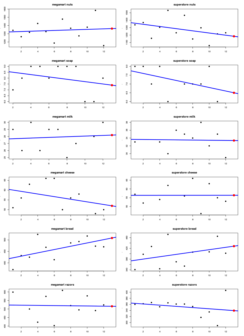
Visualized : plot
- The black dots represent the monthly sales figures.
- The blue line is the line fitted by R's lm() function through the sales dots.
- The red dot is the predicted sale for month 13.
- In each case the red dot lies on the blue line, which proves the correctness.
The R code
1 2 3 4 5 6 7 8 9 10 11 12 13 14 15 16 17 18 19 20 21 22 23 24 25 | |
Code reduction
Let's try and get rid of as many of intermediate dataframes as possible, ie. we chain as many as possible transformations together, and we skip the cosmetics (ie. rounding off).
Then the calculation of the omega's can be nicely reduced as follows ..
Starting with sale_narrow_df
sale_narrow_df.orderBy("shop","product","x").show()

+--------+-------+---+---+
|    shop|product|  x|  y|
+--------+-------+---+---+
|megamart|  bread|  1|371|
|megamart|  bread|  2|432|
|megamart|  bread|  3|425|
|megamart|  bread|  4|524|
|megamart|  bread|  5|468|
|megamart|  bread|  6|414|
..
..
Reduced number of transformations
    val avg_df = sale_narrow_df.
                        groupBy("shop","product").agg( avg("x"), avg("y") ).
                        select("shop","product","avg(x)","avg(y)")

    val coeff_df = sale_narrow_df.
                        join( avg_df, Seq("shop","product"), "leftouter").
                        withColumn("xdif", col("x")-col("avg(x)")).
                        withColumn("ydif", col("y")-col("avg(y)")).
                        withColumn("pxy", col("xdif")*col("ydif") ).
                        withColumn("pxx", col("xdif")*col("xdif") ).
                        groupBy("shop","product").agg( sum("pxy"), sum("pxx") ).
                        withColumn("w1", col("sum(pxy)")/col("sum(pxx)") ).
                        join( avg_df, Seq("shop","product"), "leftouter").
                        withColumn("w0", col("avg(y)") - col("w1") * col("avg(x)") ).
                        select("shop","product","w0","w1")
Result
coeff_df.orderBy("shop","product").show()

+----------+-------+------------------+--------------------+
|      shop|product|                w0|                  w1|
+----------+-------+------------------+--------------------+
|  megamart|  bread|414.89044585987256|   7.185987261146498|
|  megamart| cheese| 60.70096463022508| -0.6720257234726686|
|  megamart|   milk|27.585414585414583|0.046953046953046945|
|  megamart|   nuts| 1320.439393939394|   3.265734265734265|
|  megamart| razors| 523.5142857142856| -0.5744360902255637|
|  megamart|   soap|               8.7|                -0.1|
|superstore|  bread| 371.2369826435247|   4.382510013351134|
|superstore| cheese| 56.37858805275407|0.003103180760279275|
|superstore|   milk| 33.67531219980788|-0.02401536983669...|
|superstore|   nuts| 1374.439393939394| -14.657342657342657|
|superstore| razors|365.28787878787875|  -1.993006993006993|
|superstore|   soap| 7.800000000000001|                -0.1|
+----------+-------+------------------+--------------------+
Alternative
This alternative has one join less: the averages are carried over in the agg( .. ,max("avg(x)"), max("avg(y)")) :
    val coeff_df = sale_narrow_df.join( avg_df, Seq("shop","product"), "leftouter").
                          withColumn("xdif", col("x")-col("avg(x)")).
                          withColumn("ydif", col("y")-col("avg(y)")).
                          withColumn("pxy", col("xdif")*col("ydif") ).
                          withColumn("pxx", col("xdif")*col("xdif") ).
                          groupBy("shop","product").agg( sum("pxy"), sum("pxx"), max("avg(x)"), max("avg(y)") ).
                          withColumn("w1", col("sum(pxy)")/col("sum(pxx)") ).
                          withColumn("w0", col("max(avg(y))") - col("w1") * col("max(avg(x))") ).
select("shop","product","w0","w1")Turn narrow dataframe into wide
Just for matter of completeness, here a way of turning the narrow dataframe back into a wide one.
We have this narrow dataframe:
sale_narrow_df.show()

+----------+-------+---+----+
|      shop|product|  x|   y|
+----------+-------+---+----+
|superstore|  bread|  1| 341|
|superstore| cheese|  1|  57|
|superstore| razors|  1| 360|
|superstore|   soap|  1|   8|
|superstore|   milk|  1|  33|
|superstore|   nuts|  1|1338|
|  megamart|  bread|  1| 371|
|  megamart| cheese|  1|  51|
|  megamart| razors|  1| 599|
|  megamart|   nuts|  1|1342|
|superstore|  bread|  2| 398|
|superstore| cheese|  2|  52|
|superstore| razors|  2| 362|
|superstore|   soap|  2|   8|
|superstore|   nuts|  2|1369|
|  megamart|  bread|  2| 432|
|  megamart| cheese|  2|  56|
|  megamart|   soap|  2|   7|
|  megamart|   milk|  2|  29|
|  megamart|   nuts|  2|1264|
+----------+-------+---+----+
And here's a way to turn it back into a wide frame:
Step 1: create a list of dataframes, one per month
val months=Array("jan","feb","mar","apr","may","jun","jul","aug","sep","oct","nov","dec")

def sel( mon:Int, colname:String) = {
        sale_narrow_df.where(s"x=$mon").select("shop","product","y").
                       withColumnRenamed("y",colname)
}

val df_ls = for ( i <- 0 until months.length ) yield { sel(i+1, months(i) ) }
Step 2: join the list of dataframes on columns 'shop' and 'product' :
def jn(df1: org.apache.spark.sql.DataFrame, df2:org.apache.spark.sql.DataFrame) = {
    df1.join(df2,Seq("shop","product"), "outer")
}

val wide_df=df_ls.reduce( jn(_,_) )
Et voila:
wide_df.orderBy("shop","product").show()

+----------+-------+----+----+----+----+----+----+----+----+----+----+----+----+
|      shop|product| jan| feb| mar| apr| may| jun| jul| aug| sep| oct| nov| dec|
+----------+-------+----+----+----+----+----+----+----+----+----+----+----+----+
|  megamart|  bread| 371| 432| 425| 524| 468| 414|null| 487| 493| 517| 473| 470|
|  megamart| cheese|  51|  56|  63|null|  66|  66|  50|  56|  58|null|  48|  50|
|  megamart|   milk|null|  29|  26|  30|  26|  29|  29|  25|  27|null|  28|  30|
|  megamart|   nuts|1342|1264|1317|1425|1326|1187|1478|1367|1274|1380|1584|1156|
|  megamart| razors| 599|null| 500| 423| 574| 403| 609| 520| 495| 577| 491| 524|
|  megamart|   soap|null|   7|   8|   9|   9|   8|   9|   9|   9|   6|   6|   8|
|superstore|  bread| 341| 398| 427| 344| 472| 370| 354| 406|null| 407| 465| 402|
|superstore| cheese|  57|  52|null|  54|  62|null|  56|  66|  46|  63|  55|  53|
|superstore|   milk|  33|null|null|  33|  30|  36|  35|  34|  38|  32|  35|  29|
|superstore|   nuts|1338|1369|1157|1305|1532|1231|1466|1148|1298|1059|1216|1231|
|superstore| razors| 360| 362| 366| 352| 365| 361| 361| 353| 317| 335| 290| 406|
|superstore|   soap|   8|   8|   7|   8|   6|null|   7|   7|   7|   8|   6|null|
+----------+-------+----+----+----+----+----+----+----+----+----+----+----+----+Creation of random data
This R script was used to generated the random sales data.
set.seed(29.02)

# per product multiplication factor
z0=c( 10, 1, 8, 0.3, 0.5, 20)
z=c(z0,z0)

m<-matrix(0,12,12)
for ( i in 1:12) {
    mu=3*(8+round(rnorm(1,10,4))) * z[i]
    m[i,]=matrix(round(rnorm(12,mu,mu/10),0),1, 12)
}
df<- cbind( data.frame( cbind( rep(c("superstore", "megamart"),1,each=6),
                               c("bread","cheese","razors","soap","milk","nuts")) ),
            data.frame(m) )

months=c("jan","feb","mar","apr","may","jun","jul","aug","sep","oct","nov","dec")
colnames(df)= c("shop","product", months)

# punch some holes! -> ie. fill some positions with NA
num_na=15
c=2+sample(12,num_na,replace=T)
r=sample(12,num_na,replace=T)
for (i in 1:num_na ) { df[r[i],c[i]]=NA }

write.table(df, "sales.csv", row.names=F, col.names=T, sep=",", na="null", quote=T)
The output, in file "sales.csv", is copy/pasted and massaged a bit, and then fitted into the following scala script.
Create the sale_df dataframe
import org.apache.spark.sql.Row
import org.apache.spark.sql.types._
import scala.collection.JavaConversions._   // IMPORTANT !!

val sx= new org.apache.spark.sql.SQLContext(sc)

val sale_schema = StructType(
      StructField("shop",StringType,false)  ::
      StructField("product",StringType,false)  ::
      StructField("jan",IntegerType,true)  ::
      StructField("feb",IntegerType,true)  ::
      StructField("mar",IntegerType,true)  ::
      StructField("apr",IntegerType,true)  ::
      StructField("may",IntegerType,true)  ::
      StructField("jun",IntegerType,true)  ::
      StructField("jul",IntegerType,true)  ::
      StructField("aug",IntegerType,true)  ::
      StructField("sep",IntegerType,true)  ::
      StructField("oct",IntegerType,true)  ::
      StructField("nov",IntegerType,true)  ::
      StructField("dec",IntegerType,true) :: Nil
    )

val sale_df=sx.createDataFrame( new java.util.ArrayList[org.apache.spark.sql.Row]( Seq(
    Row("superstore","bread",341,398,427,344,472,370,354,406,null,407,465,402),
    Row("superstore","cheese",57,52,null,54,62,null,56,66,46,63,55,53),
    Row("superstore","razors",360,362,366,352,365,361,361,353,317,335,290,406),
    Row("superstore","soap",8,8,7,8,6,null,7,7,7,8,6,null),
    Row("superstore","milk",33,null,null,33,30,36,35,34,38,32,35,29),
    Row("superstore","nuts",1338,1369,1157,1305,1532,1231,1466,1148,1298,1059,1216,1231),
    Row("megamart","bread",371,432,425,524,468,414,null,487,493,517,473,470),
    Row("megamart","cheese",51,56,63,null,66,66,50,56,58,null,48,50),
    Row("megamart","razors",599,null,500,423,574,403,609,520,495,577,491,524),
    Row("megamart","soap",null,7,8,9,9,8,9,9,9,6,6,8),
    Row("megamart","milk",null,29,26,30,26,29,29,25,27,null,28,30),
    Row("megamart","nuts",1342,1264,1317,1425,1326,1187,1478,1367,1274,1380,1584,1156))) , sale_schema)
After running the above scala script in the Spark Shell you have the same "sale_df" used in above text.
Sidenote
In some texts you see dataframes created without defining a schema, like this:
val sale_df=sx.createDataFrame(Seq(
("superstore","bread",53,57,58,57,53,57,56,57,53,53,52,62),
("superstore","cheese",60,57,48,56,89,54,66,64,55,61,59,65),
..
..
("superstore","nuts",37,40,39,38,37,41,42,42,39,38,42,46))).toDF(
    "shop","product","jan","feb","mar","apr","may","jun","jul","aug","sep","oct","nov","dec")
That is also possible, but won't work in the above case, because we have NULLs in our data.
The aardvark.code file
The scala and R code for creating, manipulating and plotting the data in 1 neat aardvark.code file.