Convert a Garmin .FIT file and plot the heartrate of your run

Use gpsbabel to turn your FIT file into CSV:

gpsbabel -t -i garmin_fit -f 97D54119.FIT -o unicsv -F 97D54119.csv

Pandas imports:

import pandas as pd
import math
import matplotlib.pyplot as plt

pd.options.display.width=150

Read the CSV file:

df=pd.read_csv('97D54119.csv',sep=',',skip_blank_lines=False)

Show some points:

df.head(500).tail(10)


      No   Latitude  Longitude  Altitude  Speed  Heartrate  Cadence        Date      Time
490  491  50.855181   4.826737      78.2   2.79        144     78.0  2019/07/13  06:44:22
491  492  50.855136   4.826739      77.6   2.79        147     78.0  2019/07/13  06:44:24
492  493  50.854962   4.826829      76.2   2.77        148     77.0  2019/07/13  06:44:32
493  494  50.854778   4.826951      77.4   2.77        146     78.0  2019/07/13  06:44:41
494  495  50.854631   4.827062      78.0   2.71        143     78.0  2019/07/13  06:44:49
495  496  50.854531   4.827174      79.2   2.70        146     77.0  2019/07/13  06:44:54
496  497  50.854472   4.827249      79.2   2.73        149     77.0  2019/07/13  06:44:57
497  498  50.854315   4.827418      79.8   2.74        149     76.0  2019/07/13  06:45:05
498  499  50.854146   4.827516      77.4   2.67        147     76.0  2019/07/13  06:45:14
499  500  50.853985   4.827430      79.0   2.59        144     75.0  2019/07/13  06:45:22

Function to compute the distance (approximately) :

#  function to approximately calculate the distance between 2 points
#  from: http://www.movable-type.co.uk/scripts/latlong.html
def rough_distance(lat1, lon1, lat2, lon2):
    lat1 = lat1 * math.pi / 180.0
    lon1 = lon1 * math.pi / 180.0
    lat2 = lat2 * math.pi / 180.0
    lon2 = lon2 * math.pi / 180.0
    r = 6371.0 #// km
    x = (lon2 - lon1) * math.cos((lat1+lat2)/2)
    y = (lat2 - lat1)
    d = math.sqrt(x*x+y*y) * r
    return d

Compute the distance:

ds=[]
(d,priorlat,priorlon)=(0.0, 0.0, 0.0)
for t in df[['Latitude','Longitude']].itertuples():
    if len(ds)>0:
        d+=rough_distance(t.Latitude,t.Longitude, priorlat, priorlon)
    ds.append(d)
    (priorlat,priorlon)=(t.Latitude,t.Longitude)
 
df['CumulativeDist']=ds  

Let's plot!

df.plot(kind='line',x='CumulativeDist',y='Heartrate',color='red')
plt.show()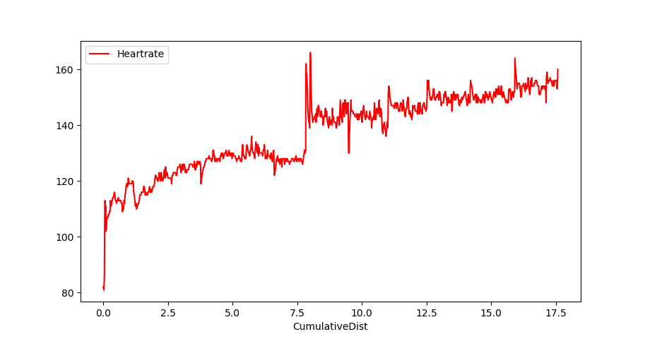 

Or multiple columns:

plt.plot( df.CumulativeDist, df.Heartrate, color='red')
plt.plot( df.CumulativeDist, df.Altitude, color='blue')
plt.show()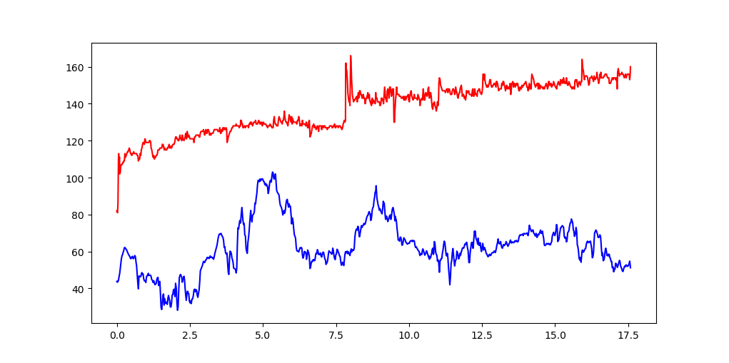

Turn a dataframe into an array

eg. dataframe cn

cn

                     asciiname  population  elevation
128677                Crossett        5507         58
7990    Santa Maria da Vitoria       23488        438
25484                 Shanling           0        628
95882     Colonia Santa Teresa       36845       2286
38943                 Blomberg        1498          4
7409              Missao Velha       13106        364
36937                  Goerzig        1295         81

Turn into an arrary

cn.iloc[range(len(cn))].values


array([['Yuhu', 0, 15],
       ['Traventhal', 551, 42],
       ['Velabisht', 0, 60],
       ['Almorox', 2319, 539],
       ['Abuyog', 15632, 6],
       ['Zhangshan', 0, 132],
       ['Llica de Vall', 0, 136],
       ['Capellania', 2252, 31],
       ['Mezocsat', 6519, 91],
       ['Vars', 1634, 52]], dtype=object)

Sidenote: cn was pulled from city data: cn=df.sample(7)[['asciiname','population','elevation']].

Turn a pandas dataframe into a dictionary

eg. create a mapping of a 3 digit code to a country name

BEL -> Belgium
CHN -> China
FRA -> France
..

Code:

df=pd.io.parsers.read_table(
    '/u01/data/20150215_country_code_iso/country_codes.txt',
    sep='|')

c3d=df.set_index('c3')['country'].to_dict()

Result:

c3d['AUS']
'Australia'

c3d['GBR']
'United Kingdom'

eg. read a csv file that has nasty quotes, and save it as tab-separated.

import pandas as pd
import csv

colnames= ["userid", "movieid", "tag", "timestamp"]

df=pd.io.parsers.read_table("tags.csv",
                sep=",", header=0, names= colnames,
                quoting=csv.QUOTE_ALL)

Write:

df.to_csv('tags.tsv', index=False, sep='\t')

Dataframe aggregation fun

Load the city dataframe into dataframe df.

Summary statistic of 1 column

df.population.describe()

count    2.261100e+04
mean     1.113210e+05
std      4.337739e+05
min      0.000000e+00
25%      2.189950e+04
50%      3.545000e+04
75%      7.402450e+04
max      1.460851e+07

Summary statistic per group

Load the city dataframe into df, then:

t1=df[['country','population']].groupby(['country'])
t2=t1.agg( ['min','mean','max','count'])
t2.sort_values(by=[ ('population','count') ],ascending=False).head(20)

Output:

        population                               
               min           mean       max count
country                                          
US           15002   62943.294138   8175133  2900
IN           15007  109181.708924  12691836  2398
BR               0  104364.320502  10021295  1195
DE               0   57970.979716   3426354   986
RU           15048  101571.065195  10381222   951
CN           15183  357967.030457  14608512   788
JP           15584  136453.906915   8336599   752
IT             895   49887.442136   2563241   674
GB           15024   81065.611200   7556900   625
FR           15009   44418.920455   2138551   616
ES           15006   65588.432282   3255944   539
MX           15074  153156.632735  12294193   501
PH           15066  100750.534884  10444527   430
TR           15058  142080.305263  11174257   380
ID           17504  170359.848901   8540121   364
PL           15002   64935.379421   1702139   311
PK           15048  160409.378641  11624219   309
NL           15071   53064.727626    777725   257
UA           15012  103468.816000   2514227   250
NG           15087  205090.336207   9000000   232

Note on selecting a multilevel column

Eg. select 'min' via tuple ('population','min').

t2[ t2[('population','min')]>50000 ]

        population                             
               min          mean      max count
country                                        
BB           98511  9.851100e+04    98511     1
CW          125000  1.250000e+05   125000     1
HK          288728  3.107000e+06  7012738     3
MO          520400  5.204000e+05   520400     1
MR           72337  3.668685e+05   661400     2
MV          103693  1.036930e+05   103693     1
SB           56298  5.629800e+04    56298     1
SG         3547809  3.547809e+06  3547809     1
ST           53300  5.330000e+04    53300     1
TL          150000  1.500000e+05   150000     1

Turn a dataframe into sql statements

The easiest way is to go via sqlite!

eg. the two dataframes udf and tdf.

import sqlite3
con=sqlite3.connect('txdb.sqlite') 
udf.to_sql(name='t_user', con=con, index=False)
tdf.to_sql(name='t_transaction', con=con, index=False)
con.close()

Then on the command line:

sqlite3 txdb.sqlite .dump > create.sql 

This is the created create.sql script:

PRAGMA foreign_keys=OFF;
BEGIN TRANSACTION;

CREATE TABLE "t_user" (
"uid" INTEGER,
  "name" TEXT
);
INSERT INTO "t_user" VALUES(9000,'Gerd Abrahamsson');
INSERT INTO "t_user" VALUES(9001,'Hanna Andersson');
INSERT INTO "t_user" VALUES(9002,'August Bergsten');
INSERT INTO "t_user" VALUES(9003,'Arvid Bohlin');
INSERT INTO "t_user" VALUES(9004,'Edvard Marklund');
INSERT INTO "t_user" VALUES(9005,'Ragnhild Brännström');
INSERT INTO "t_user" VALUES(9006,'Börje Wallin');
INSERT INTO "t_user" VALUES(9007,'Otto Byström');
INSERT INTO "t_user" VALUES(9008,'Elise Dahlström');

CREATE TABLE "t_transaction" (
"xid" INTEGER,
  "uid" INTEGER,
  "amount" INTEGER,
  "date" TEXT
);
INSERT INTO "t_transaction" VALUES(5000,9008,498,'2016-02-21 06:28:49');
INSERT INTO "t_transaction" VALUES(5001,9003,268,'2016-01-17 13:37:38');
INSERT INTO "t_transaction" VALUES(5002,9003,621,'2016-02-24 15:36:53');
INSERT INTO "t_transaction" VALUES(5003,9007,-401,'2016-01-14 16:43:27');
INSERT INTO "t_transaction" VALUES(5004,9004,720,'2016-05-14 16:29:54');
INSERT INTO "t_transaction" VALUES(5005,9007,-492,'2016-02-24 23:58:57');
INSERT INTO "t_transaction" VALUES(5006,9002,-153,'2016-02-18 17:58:33');
INSERT INTO "t_transaction" VALUES(5007,9008,272,'2016-05-26 12:00:00');
INSERT INTO "t_transaction" VALUES(5008,9005,-250,'2016-02-24 23:14:52');
INSERT INTO "t_transaction" VALUES(5009,9008,82,'2016-04-20 18:33:25');
INSERT INTO "t_transaction" VALUES(5010,9006,549,'2016-02-16 14:37:25');
INSERT INTO "t_transaction" VALUES(5011,9008,-571,'2016-02-28 13:05:33');
INSERT INTO "t_transaction" VALUES(5012,9008,814,'2016-03-20 13:29:11');
INSERT INTO "t_transaction" VALUES(5013,9005,-114,'2016-02-06 14:55:10');
INSERT INTO "t_transaction" VALUES(5014,9005,819,'2016-01-18 10:50:20');
INSERT INTO "t_transaction" VALUES(5015,9001,-404,'2016-02-20 22:08:23');
INSERT INTO "t_transaction" VALUES(5016,9000,-95,'2016-05-09 10:26:05');
INSERT INTO "t_transaction" VALUES(5017,9003,428,'2016-03-27 15:30:47');
INSERT INTO "t_transaction" VALUES(5018,9002,-549,'2016-04-15 21:44:49');
INSERT INTO "t_transaction" VALUES(5019,9001,-462,'2016-03-09 20:32:35');
INSERT INTO "t_transaction" VALUES(5020,9004,-339,'2016-05-03 17:11:21');
COMMIT;

The script doesn't create the indexes (because of Index='False'), so here are the statements:

CREATE INDEX "ix_t_user_uid" ON "t_user" ("uid");
CREATE INDEX "ix_t_transaction_xid" ON "t_transaction" ("xid");

Or better: create primary keys on those tables!

Join two dataframes, sql style

You have a number of users, and a number of transactions against those users. Join these 2 dataframes.

import pandas as pd 

User dataframe

ids= [9000, 9001, 9002, 9003, 9004, 9005, 9006, 9007, 9008]
nms=[u'Gerd Abrahamsson', u'Hanna Andersson', u'August Bergsten',
      u'Arvid Bohlin', u'Edvard Marklund', u'Ragnhild Br\xe4nnstr\xf6m',
      u'B\xf6rje Wallin', u'Otto Bystr\xf6m',u'Elise Dahlstr\xf6m']


udf=pd.DataFrame(ids, columns=['uid'])
udf['name']=nms

Content of udf:

    uid                 name
0  9000     Gerd Abrahamsson
1  9001      Hanna Andersson
2  9002      August Bergsten
3  9003         Arvid Bohlin
4  9004      Edvard Marklund
5  9005  Ragnhild Brännström
6  9006         Börje Wallin
7  9007         Otto Byström
8  9008      Elise Dahlström

Transaction dataframe

tids= [5000, 5001, 5002, 5003, 5004, 5005, 5006, 5007, 5008, 5009, 5010, 5011, 5012,
       5013, 5014, 5015, 5016, 5017, 5018, 5019, 5020]

uids= [9008, 9003, 9003, 9007, 9004, 9007, 9002, 9008, 9005, 9008, 9006, 9008, 9008,
       9005, 9005, 9001, 9000, 9003, 9002, 9001, 9004] 

tamt= [498, 268, 621, -401, 720, -492, -153, 272, -250, 82, 549, -571, 814, -114,
      819, -404, -95, 428, -549, -462, -339]

tdt= ['2016-02-21 06:28:49', '2016-01-17 13:37:38', '2016-02-24 15:36:53',
      '2016-01-14 16:43:27', '2016-05-14 16:29:54', '2016-02-24 23:58:57',
      '2016-02-18 17:58:33', '2016-05-26 12:00:00', '2016-02-24 23:14:52',
      '2016-04-20 18:33:25', '2016-02-16 14:37:25', '2016-02-28 13:05:33',
      '2016-03-20 13:29:11', '2016-02-06 14:55:10', '2016-01-18 10:50:20',
      '2016-02-20 22:08:23', '2016-05-09 10:26:05', '2016-03-27 15:30:47',
      '2016-04-15 21:44:49', '2016-03-09 20:32:35', '2016-05-03 17:11:21']


tdf=pd.DataFrame(tids, columns=['xid'])
tdf['uid']=uids
tdf['amount']=tamt
tdf['date']=tdt

Content of tdf:

     xid   uid  amount                 date
0   5000  9008     498  2016-02-21 06:28:49
1   5001  9003     268  2016-01-17 13:37:38
2   5002  9003     621  2016-02-24 15:36:53
3   5003  9007    -401  2016-01-14 16:43:27
4   5004  9004     720  2016-05-14 16:29:54
5   5005  9007    -492  2016-02-24 23:58:57
6   5006  9002    -153  2016-02-18 17:58:33
7   5007  9008     272  2016-05-26 12:00:00
8   5008  9005    -250  2016-02-24 23:14:52
9   5009  9008      82  2016-04-20 18:33:25
10  5010  9006     549  2016-02-16 14:37:25
11  5011  9008    -571  2016-02-28 13:05:33
12  5012  9008     814  2016-03-20 13:29:11
13  5013  9005    -114  2016-02-06 14:55:10
14  5014  9005     819  2016-01-18 10:50:20
15  5015  9001    -404  2016-02-20 22:08:23
16  5016  9000     -95  2016-05-09 10:26:05
17  5017  9003     428  2016-03-27 15:30:47
18  5018  9002    -549  2016-04-15 21:44:49
19  5019  9001    -462  2016-03-09 20:32:35
20  5020  9004    -339  2016-05-03 17:11:21

Join sql-style: pd.merge

pd.merge( tdf, udf, how='inner', left_on='uid', right_on='uid')

     xid   uid  amount                 date                 name
0   5000  9008     498  2016-02-21 06:28:49      Elise Dahlström
1   5007  9008     272  2016-05-26 12:00:00      Elise Dahlström
2   5009  9008      82  2016-04-20 18:33:25      Elise Dahlström
3   5011  9008    -571  2016-02-28 13:05:33      Elise Dahlström
4   5012  9008     814  2016-03-20 13:29:11      Elise Dahlström
5   5001  9003     268  2016-01-17 13:37:38         Arvid Bohlin
6   5002  9003     621  2016-02-24 15:36:53         Arvid Bohlin
7   5017  9003     428  2016-03-27 15:30:47         Arvid Bohlin
8   5003  9007    -401  2016-01-14 16:43:27         Otto Byström
9   5005  9007    -492  2016-02-24 23:58:57         Otto Byström
10  5004  9004     720  2016-05-14 16:29:54      Edvard Marklund
11  5020  9004    -339  2016-05-03 17:11:21      Edvard Marklund
12  5006  9002    -153  2016-02-18 17:58:33      August Bergsten
13  5018  9002    -549  2016-04-15 21:44:49      August Bergsten
14  5008  9005    -250  2016-02-24 23:14:52  Ragnhild Brännström
15  5013  9005    -114  2016-02-06 14:55:10  Ragnhild Brännström
16  5014  9005     819  2016-01-18 10:50:20  Ragnhild Brännström
17  5010  9006     549  2016-02-16 14:37:25         Börje Wallin
18  5015  9001    -404  2016-02-20 22:08:23      Hanna Andersson
19  5019  9001    -462  2016-03-09 20:32:35      Hanna Andersson
20  5016  9000     -95  2016-05-09 10:26:05     Gerd Abrahamsson

Sidenote: fake data creation

This is the way the above fake data was created:

import random
from faker import Factory

fake = Factory.create('sv_SE') 

ids=[]
nms=[]
for i in range(0,9):
    ids.append(9000+i)
    nms.append(fake.name())
    print "%d\t%s" % ( ids[i],nms[i])


tids=[]
uids=[]
tamt=[]
tdt=[]
sign=[-1,1]
for i in range(0,21):
    tids.append(5000+i)
    tamt.append(sign[random.randint(0,1)]*random.randint(80,900))
    uids.append(ids[random.randint(0,len(ids)-1)])
    tdt.append(str(fake.date_time_this_year()))
    print "%d\t%d\t%d\t%s" % ( tids[i], tamt[i], uids[i], tdt[i])

Read data from a zipfile into a dataframe

import pandas as pd
import zipfile

z = zipfile.ZipFile("lending-club-data.csv.zip")
df=pd.io.parsers.read_table(z.open("lending-club-data.csv"), sep=",") 
z.close()

Calculate the cumulative distance of gps trackpoints

Prep:

import pandas as pd
import math

Function to calculate the distance:

#  function to approximately calculate the distance between 2 points
#  from: http://www.movable-type.co.uk/scripts/latlong.html
def rough_distance(lat1, lon1, lat2, lon2):
    lat1 = lat1 * math.pi / 180.0
    lon1 = lon1 * math.pi / 180.0
    lat2 = lat2 * math.pi / 180.0
    lon2 = lon2 * math.pi / 180.0
    r = 6371.0 #// km
    x = (lon2 - lon1) * math.cos((lat1+lat2)/2)
    y = (lat2 - lat1)
    d = math.sqrt(x*x+y*y) * r
    return d

Read data:

df=pd.io.parsers.read_table("trk.tsv",sep="\t")

# drop some columns (for clarity) 
df=df.drop(['track','ele','tm_str'],axis=1) 

Sample:

df.head()

         lat       lon
0  50.848408  4.787456
1  50.848476  4.787367
2  50.848572  4.787275
3  50.848675  4.787207
4  50.848728  4.787189

The prior-latitude column is the latitude column shifted by 1 unit:

df['prior_lat']= df['lat'].shift(1)
prior_lat_ix=df.columns.get_loc('prior_lat')
df.iloc[0,prior_lat_ix]= df.lat.iloc[0]

The prior-longitude column is the longitude column shifted by 1 unit:

df['prior_lon']= df['lon'].shift(1)
prior_lon_ix=df.columns.get_loc('prior_lon')
df.iloc[0,prior_lon_ix]= df.lon.iloc[0]

Calculate the distance:

df['dist']= df[ ['lat','lon','prior_lat','prior_lon'] ].apply(
                        lambda r : rough_distance ( r[0], r[1], r[2], r[3]) , axis=1)

Calculate the cumulative distance

cum=0
cum_dist=[]
for d in df['dist']:
    cum=cum+d
    cum_dist.append(cum)

df['cum_dist']=cum_dist

Sample:

df.head()

         lat       lon  prior_lat  prior_lon      dist  cum_dist
0  50.848408  4.787456  50.848408   4.787456  0.000000  0.000000
1  50.848476  4.787367  50.848408   4.787456  0.009831  0.009831
2  50.848572  4.787275  50.848476   4.787367  0.012435  0.022266
3  50.848675  4.787207  50.848572   4.787275  0.012399  0.034665
4  50.848728  4.787189  50.848675   4.787207  0.006067  0.040732



df.tail()

            lat       lon  prior_lat  prior_lon      dist   cum_dist
1012  50.847164  4.788163  50.846962   4.788238  0.023086  14.937470
1013  50.847267  4.788134  50.847164   4.788163  0.011634  14.949104
1014  50.847446  4.788057  50.847267   4.788134  0.020652  14.969756
1015  50.847630  4.787978  50.847446   4.788057  0.021097  14.990853
1016  50.847729  4.787932  50.847630   4.787978  0.011496  15.002349

Onehot encode the categorical data of a data-frame

.. using the pandas get_dummies function.

Data:

import StringIO
import pandas as pd

data_strio=StringIO.StringIO('''category   reason         species
Decline    Genuine        24
Improved   Genuine        16
Improved   Misclassified  85
Decline    Misclassified  41
Decline    Taxonomic      2
Improved   Taxonomic      7
Decline    Unclear        41
Improved   Unclear        117''')

df=pd.read_fwf(data_strio)

One hot encode 'category':

cat_oh= pd.get_dummies(df['category'])
cat_oh.columns= map( lambda x: "cat__"+x.lower(), cat_oh.columns.values)

cat_oh

   cat__decline  cat__improved
0             1              0
1             0              1
2             0              1
3             1              0
4             1              0
5             0              1
6             1              0
7             0              1

Do the same for 'reason' :

reason_oh= pd.get_dummies(df['reason'])
reason_oh.columns= map( lambda x: "rsn__"+x.lower(), reason_oh.columns.values)

Combine

Combine the columns into a new dataframe:

ohdf= pd.concat( [ cat_oh, reason_oh, df['species']], axis=1)

Result:

ohdf

   cat__decline  cat__improved  rsn__genuine  rsn__misclassified  \
0             1              0             1                   0   
1             0              1             1                   0   
2             0              1             0                   1   
3             1              0             0                   1   
4             1              0             0                   0   
5             0              1             0                   0   
6             1              0             0                   0   
7             0              1             0                   0   

   rsn__taxonomic  rsn__unclear  species  
0               0             0       24  
1               0             0       16  
2               0             0       85  
3               0             0       41  
4               1             0        2  
5               1             0        7  
6               0             1       41  
7               0             1      117  

Or if the 'drop' syntax on the dataframe is more convenient to you:

ohdf= pd.concat( [ cat_oh, reason_oh, 
            df.drop(['category','reason'], axis=1) ], 
            axis=1)

Read a fixed-width datafile inline

import StringIO
import pandas as pd

data_strio=StringIO.StringIO('''category   reason         species
Decline    Genuine        24
Improved   Genuine        16
Improved   Misclassified  85
Decline    Misclassified  41
Decline    Taxonomic      2
Improved   Taxonomic      7
Decline    Unclear        41
Improved   Unclear        117''')

Turn the string_IO into a dataframe:

df=pd.read_fwf(data_strio)

Check the content:

df

   category         reason  species
0   Decline        Genuine       24
1  Improved        Genuine       16
2  Improved  Misclassified       85
3   Decline  Misclassified       41
4   Decline      Taxonomic        2
5  Improved      Taxonomic        7
6   Decline        Unclear       41
7  Improved        Unclear      117

The "5-number" summary

df.describe()

          species
count    8.000000
mean    41.625000
std     40.177952
min      2.000000
25%     13.750000
50%     32.500000
75%     52.000000
max    117.000000

Drop a column

df=df.drop('reason',axis=1) 

Result:

   category  species
0   Decline       24
1  Improved       16
2  Improved       85
3   Decline       41
4   Decline        2
5  Improved        7
6   Decline       41
7  Improved      117

Add/subtract a delta time

Problem

A number of photo files were tagged as follows, with the date and the time:

20151205_17h48-img_0098.jpg
20151205_18h20-img_0099.jpg
20151205_18h21-img_0100.jpg

..

Turns out that they should be all an hour earlier (reminder: mixing pics from two camera's), so let's create a script to rename these files...

Solution

1. Start

Let's use pandas:

import datetime as dt
import pandas as pd
import re

df0=pd.io.parsers.read_table( '/u01/work/20151205_gran_canaria/fl.txt',sep=",", \
        header=None, names= ["fn"])
df=df0[df0['fn'].apply( lambda a: 'img_0' in a )]  # filter out certain pics     

2. Make parseable

Now add a column to the dataframe that only contains the numbers of the date, so it can be parsed:

df['rawdt']=df['fn'].apply( lambda a: re.sub('-.*.jpg','',a))\
                 .apply( lambda a: re.sub('[_h]','',a))

Result:

df.head()
                             fn         rawdt
0   20151202_07h17-img_0001.jpg  201512020717
1   20151202_07h17-img_0002.jpg  201512020717
2   20151202_07h17-img_0003.jpg  201512020717
3   20151202_15h29-img_0004.jpg  201512021529
28  20151202_17h59-img_0005.jpg  201512021759

3. Convert to datetime, and subtract delta time

Convert the raw-date to a real date, and subtract an hour:

df['adjdt']=pd.to_datetime( df['rawdt'], format('%Y%m%d%H%M'))-dt.timedelta(hours=1)

Note 20190105: apparently you can drop the 'format' string:

df['adjdt']=pd.to_datetime( df['rawdt'])-dt.timedelta(hours=1) 

Result:

                             fn         rawdt               adjdt
0   20151202_07h17-img_0001.jpg  201512020717 2015-12-02 06:17:00
1   20151202_07h17-img_0002.jpg  201512020717 2015-12-02 06:17:00
2   20151202_07h17-img_0003.jpg  201512020717 2015-12-02 06:17:00
3   20151202_15h29-img_0004.jpg  201512021529 2015-12-02 14:29:00
28  20151202_17h59-img_0005.jpg  201512021759 2015-12-02 16:59:00

4. Convert adjusted date to string

df['adj']=df['adjdt'].apply(lambda a: dt.datetime.strftime(a, "%Y%m%d_%Hh%M") )

We also need the 'stem' of the filename:

df['stem']=df['fn'].apply(lambda a: re.sub('^.*-','',a) )

Result:

df.head()
                             fn         rawdt               adjdt  \
0   20151202_07h17-img_0001.jpg  201512020717 2015-12-02 06:17:00   
1   20151202_07h17-img_0002.jpg  201512020717 2015-12-02 06:17:00   
2   20151202_07h17-img_0003.jpg  201512020717 2015-12-02 06:17:00   
3   20151202_15h29-img_0004.jpg  201512021529 2015-12-02 14:29:00   
28  20151202_17h59-img_0005.jpg  201512021759 2015-12-02 16:59:00   

               adj          stem  
0   20151202_06h17  img_0001.jpg  
1   20151202_06h17  img_0002.jpg  
2   20151202_06h17  img_0003.jpg  
3   20151202_14h29  img_0004.jpg  
28  20151202_16h59  img_0005.jpg  

5. Cleanup

Drop columns that are no longer useful:

df=df.drop(['rawdt','adjdt'], axis=1)

Result:

df.head()
                             fn             adj          stem
0   20151202_07h17-img_0001.jpg  20151202_06h17  img_0001.jpg
1   20151202_07h17-img_0002.jpg  20151202_06h17  img_0002.jpg
2   20151202_07h17-img_0003.jpg  20151202_06h17  img_0003.jpg
3   20151202_15h29-img_0004.jpg  20151202_14h29  img_0004.jpg
28  20151202_17h59-img_0005.jpg  20151202_16h59  img_0005.jpg

6. Generate scripts

Generate the 'rename' script:

sh=df.apply( lambda a: 'mv {} {}-{}'.format( a[0],a[1],a[2]), axis=1)
sh.to_csv('rename.sh',header=False, index=False )

Also generate the 'rollback' script (in case we have to rollback the renaming) :

sh=df.apply( lambda a: 'mv {}-{} {}'.format( a[1],a[2],a[0]), axis=1)
sh.to_csv('rollback.sh',header=False, index=False )

First lines of the rename script:

mv 20151202_07h17-img_0001.jpg 20151202_06h17-img_0001.jpg
mv 20151202_07h17-img_0002.jpg 20151202_06h17-img_0002.jpg
mv 20151202_07h17-img_0003.jpg 20151202_06h17-img_0003.jpg
mv 20151202_15h29-img_0004.jpg 20151202_14h29-img_0004.jpg
mv 20151202_17h59-img_0005.jpg 20151202_16h59-img_0005.jpg

Create an empty dataframe

10
11
12
13
14
15
16
17

# create 
df=pd.DataFrame(np.zeros(0,dtype=[
    ('ProductID', 'i4'),
    ('ProductName', 'a50')
    ]))

# append
df = df.append({'ProductID':1234, 'ProductName':'Widget'},ignore_index=True)

Other way

24
25

columns = ['price', 'item']
df2 = pd.DataFrame(data=np.zeros((0,len(columns))), columns=columns) 

Quickies

You want to pandas to print more data on your wide terminal window?

pd.set_option('display.line_width', 200)

You want to make the max column width larger?

pd.set_option('max_colwidth',80)

Dataframe with date-time index

Create a dataframe df with a datetime index and some random values: (note: see 'simpler' dataframe creation further down)

Output:

    In [4]: df.head(10)
    Out[4]: 
                value
    2009-12-01     71
    2009-12-02     92
    2009-12-03     64
    2009-12-04     55
    2009-12-05     99
    2009-12-06     51
    2009-12-07     68
    2009-12-08     64
    2009-12-09     90
    2009-12-10     57
    [10 rows x 1 columns]

Now select a week of data

Output: watchout selects 8 days!!

    In [235]: df[d1:d2]
    Out[235]: 
                value
    2009-12-10     99
    2009-12-11     70
    2009-12-12     83
    2009-12-13     90
    2009-12-14     60
    2009-12-15     64
    2009-12-16     59
    2009-12-17     97
    [8 rows x 1 columns]


    In [236]: df[d1:d1+dt.timedelta(days=7)]
    Out[236]: 
                value
    2009-12-10     99
    2009-12-11     70
    2009-12-12     83
    2009-12-13     90
    2009-12-14     60
    2009-12-15     64
    2009-12-16     59
    2009-12-17     97
    [8 rows x 1 columns]


    In [237]: df[d1:d1+dt.timedelta(weeks=1)]
    Out[237]: 
                value
    2009-12-10     99
    2009-12-11     70
    2009-12-12     83
    2009-12-13     90
    2009-12-14     60
    2009-12-15     64
    2009-12-16     59
    2009-12-17     97
    [8 rows x 1 columns]

Postscriptum: a simpler way of creating the dataframe

An index of a range of dates can also be created like this with pandas:

pd.date_range('20091201', periods=31)

Hence the dataframe:

df=pd.DataFrame(np.random.randint(50,100,31), index=pd.date_range('20091201', periods=31))

Add two dataframes

Add the contents of two dataframes, having the same index

a=pd.DataFrame( np.random.randint(1,10,5), index=['a', 'b', 'c', 'd', 'e'], columns=['val'])
b=pd.DataFrame( np.random.randint(1,10,3), index=['b', 'c', 'e'],columns=['val'])

a
   val
a    5
b    7
c    8
d    8
e    1

b
   val
b    9
c    2
e    5

a+b
   val
a  NaN
b   16
c   10
d  NaN
e    6

a.add(b,fill_value=0)
   val
a    5
b   16
c   10
d    8
e    6

Read/write csv

Read:

pd.read_csv('in.csv')

Write:

<yourdataframe>.to_csv('out.csv',header=False, index=False ) 

Load a csv file

Load the following csv file. Difficulty: the date is spread over 3 fields.

    2014, 8, 5, IBM, BUY, 50,
    2014, 10, 9, IBM, SELL, 20 ,
    2014, 9, 17, PG, BUY, 10,
    2014, 8, 15, PG, SELL, 20 ,

The way I implemented it:

10
11
12
13
14
15
16
17
18
19
20
21
22

# my way
ls_order_col= [ 'year', 'month', 'day', 'symbol', 'buy_sell', 'number','dummy' ]
df_mo=pd.read_csv(s_filename, sep=',', names=ls_order_col, skipinitialspace=True, index_col=False)

# add column of type datetime 
df_mo['date']=pd.to_datetime(df_mo.year*10000+df_mo.month*100+df_mo.day,format='%Y%m%d')

# drop some columns
df_mo.drop(['dummy','year','month','day'], axis=1, inplace=True)

# order by datetime
df_mo.sort(columns='date',inplace=True )
print df_mo

An alternative way,... it's better because the date is converted on reading, and the dataframe is indexed by the date.