Implementation of the 3 formulas

Code:

15
16
17
18
19
20
21
22
23
24
25
26
27
28
29
30
31
32
33
34
35
36
37
38
39
40

# Formula 1
xmean = sum(x_v)/len(x_v) 
ymean = sum(y_v)/len(y_v) 
wh1_f1= sum([ (xi-xmean)*(yi-ymean) for (xi,yi) in zip(x_v,y_v) ]) /  \
            sum([ (xi -xmean)**2 for xi in x_v ]) 
wh0_f1= ymean-wh1_f1*xmean 
print "Formula 1: slope={} intercept={}".format(wh1_f1,wh0_f1)


# Formula 2
n=len(x_v)
sig_y = sum(y_v)
sig_x = sum(x_v) 
sig_xy = sum( [ xi*yi for (xi,yi) in zip(x_v,y_v) ])  
sig_x2 = sum( [ xi*xi for xi in x_v ] )   
wh1_f2= (sig_xy  - (sig_y*sig_x)/n ) / ( sig_x2 - sig_x*sig_x/n) 
wh0_f2= (sig_y  - wh1_f2 * sig_x) /n 
print "Formula 2: slope={} intercept={}".format(wh1_f2,wh0_f2)


# Formula 3
# Watchout: for calculating the correlation don't use np.correlate()
# but use the pearson correlation!
wh1_f3=pearsonr( y_v, x_v)[0] * np.std(y_v)/np.std(x_v)
wh0_f3= ymean-wh1_f3*xmean 
print "Formula 3: slope={} intercept={}".format(wh1_f3,wh0_f3)

Output:

Formula 1: slope=1.53848181625 intercept=117.041068001
Formula 2: slope=1.53848181625 intercept=117.041068001
Formula 3: slope=1.53848181625 intercept=117.041068001

Use libraries

Python

You can use scipy's stats.linregress() or numpy's np.polyfit()

Code:

15
16
17
18
19
20
21

# scipy stats
wh1_l1, wh0_l1, r_value, p_value, std_err = stats.linregress(x_v,y_v)
print "Library Function 1: slope={} intercept={}".format(wh1_l1,wh0_l1)

# numpy polyfit
wh1_l2,wh0_l2=np.polyfit(x_v,y_v,1)
print "Library Function 2: slope={} intercept={}".format(wh1_l2,wh0_l2)

Output:

Library Function 1: slope=1.53848181625 intercept=117.041068001
Library Function 2: slope=1.53848181625 intercept=117.041068001

Plot the result

Plot the points plus fitted line:

    # fitted line, compute 2 points
    xl=[ 0.8*min(x_v), 1.2*max(x_v) ] 
    yl=map( lambda x: slope*x+intercept, xl) 

    plt.scatter(x_v, y_v)  # all points
    plt.plot( xl,yl, 'r')  # fitted line
    plt.show()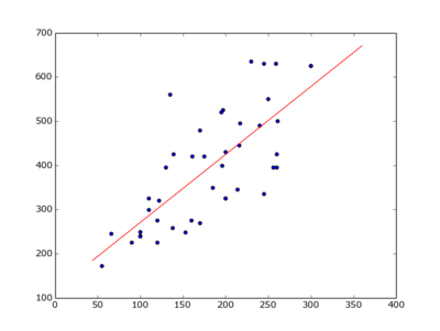

Predict the price for 100, 200 and 400 m² :

    [ (x,round(slope*x+intercept)) for x in  [100,200,400] ]

    [(100, 271.0), 
     (200, 425.0), 
     (400, 732.0)]

R implementation using lm()

First load the vectors x_v and y_v (see higher).

    df=data.frame(sqm=x_v, price=y_v)
    model=lm(price~sqm, df) 

    model$coefficients
    (Intercept)         sqm 
    117.041068    1.538482 

Plot:

    plot(price~sqm,df)
    abline(model,col="red",lwd=3)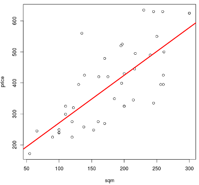

Predict the price for a 100, 200 and 400 m² house:

    predict(model, data.frame(sqm=c(100,200,400)))

           1        2        3 
    270.8892 424.7374 732.4338