x_v= [300.,245.,170.,261.,240.,200.,217.,55.,110.,256.,90.,245.,200.,
      139.,260.,300.,195.,153.,138.,185.,170.,66.,100.,160.,110.,197.,
      135.,214.,259.,196.,216.,161.,100.,130.,250.,120.,230.,122.,120.,
      260.,175.,200.,100.]

y_v= [625.,335.,479.,500.,490.,325.,495.,172.,325.,395.,225.,630.,325.,
      425.,425.,625.,520.,248.,258.,349.,269.,245.,249.,275.,299.,525.,
      560.,345.,630.,399.,445.,420.,240.,395.,550.,225.,635.,320.,275.,
395.,420.,430.,239.]Simple Linear Regression
Pages:
01_intro
02_formulas
03_data
04_implementation
05_gradient_descent
99_formulas
99_nitty_gritty
01_intro
02_formulas
03_data
04_implementation
05_gradient_descent
99_formulas
99_nitty_gritty
One Page
01_intro
20160102
Introduction
You have a bunch of related x,y coordinates (eg. the house sales in function of surface area) and you want to find out what line is a good representation of that data. Ie. you want to apply 'simple linear regression'.
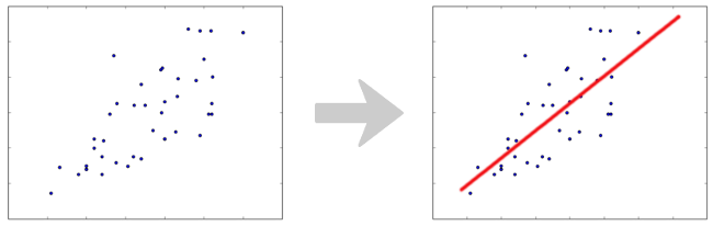
The resulting line can be represented by this function: y = w₁ x + w₀, whereby w₁ is called the slope and w₀ is the intercept.
02_formulas
20160102
Formulas
The estimated slope w₁ and intercept w₀ can be calculated using following formulas.
Formula 1

Formula 2
(derivation: see end of this article)

Formula 3
Coefficient w₁-hat expressed as a product of the correlation between y-values and x-values, and the fraction of standard-deviation of y-values over standard deviation of x-values:

Note
In above formulas read the sigma as sum from i=1 to n:

03_data
20160102
House price data
The data used is this article is the following, actual house price data sampled on 2016-01-02. The x vector has the surface area in square meters, and the y vector contains the corresponding price in kilo-EURO's.
x_v= c(300,245,170,261,240,200,217,55,110,256,90,245,200,139,260,300,
      195,153,138,185,170,66,100,160,110,197,135,214,259,196,216,161,
      100,130,250,120,230,122,120,260,175,200,100)

y_v= c(625,335,479,500,490,325,495,172,325,395,225,630,325,425,425,625,
      520,248,258,349,269,245,249,275,299,525,560,345,630,399,445,420,
      240,395,550,225,635,320,275,395,420,430,239)
Scatterplot
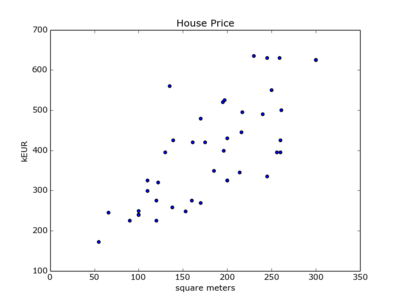
    import matplotlib.pyplot as plt

    plt.scatter(x_v, y_v)
    plt.ylabel('kEUR')
    plt.xlabel('square meters')
    plt.title('House Price')
    plt.show()
04_implementation
20160102
Implementation of the 3 formulas
Code:
15 16 17 18 19 20 21 22 23 24 25 26 27 28 29 30 31 32 33 34 35 36 37 38 39 40 | |
Output:
Formula 1: slope=1.53848181625 intercept=117.041068001
Formula 2: slope=1.53848181625 intercept=117.041068001
Formula 3: slope=1.53848181625 intercept=117.041068001
Use libraries
Python
You can use scipy's stats.linregress() or numpy's np.polyfit()
Code:
15 16 17 18 19 20 21 | |
Output:
Library Function 1: slope=1.53848181625 intercept=117.041068001
Library Function 2: slope=1.53848181625 intercept=117.041068001
Plot the result
Plot the points plus fitted line:
    # fitted line, compute 2 points
    xl=[ 0.8*min(x_v), 1.2*max(x_v) ]
    yl=map( lambda x: slope*x+intercept, xl)

    plt.scatter(x_v, y_v)  # all points
    plt.plot( xl,yl, 'r')  # fitted line
    plt.show()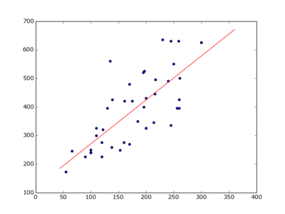
Predict the price for 100, 200 and 400 m² :
    [ (x,round(slope*x+intercept)) for x in  [100,200,400] ]

    [(100, 271.0),
     (200, 425.0),
     (400, 732.0)]
R implementation using lm()
First load the vectors x_v and y_v (see higher).
    df=data.frame(sqm=x_v, price=y_v)
    model=lm(price~sqm, df)

    model$coefficients
    (Intercept)         sqm
    117.041068    1.538482
Plot:
    plot(price~sqm,df)
    abline(model,col="red",lwd=3)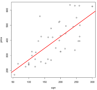
Predict the price for a 100, 200 and 400 m² house:
    predict(model, data.frame(sqm=c(100,200,400)))

           1        2        3
    270.8892 424.7374 732.4338
99_formulas
20160102
Formula 2
How to derive the above mentioned formula 2:

99_nitty_gritty
20160102
Formula 2 derivation
How to derive the above mentioned formula 2:
05_gradient_descent
20160120
Gradient descent
Minimize the Residual Sum of Squares
The slope & intercept can also be found via minimizing the RSS, which is a function of the slope (w₁) and intercept (w₀):

Finding the minimum or maximum corresponds to setting the derived function equal to zero.
KLAD For a concave or convex function there is only one point where there is a maximum or minimum, ie where the derivative equals zero. If a function is not concave nor convex, then it may have multiple maxima or minima.
Side-step: hill descent
The gradient descent algorithm tries to find a minimum, in a step-wise fashion. This can easily be compared to the following hill descent for a simple parabole function, eg. y = 5 + (x-10)².
Hill descent with overshoot
Suppose you start at point x=1. To see if the function is going down or up we add a minute quantity, dx, and know that we are descending if f(x) > fx(x+dx).
Increment x with step=15.0, and look again at the direction in which the function is going. Here the direction has flipped, we have overshot our target, so for the next step we need to divide the step-size into half. Etc.
Keep doing this until the difference is smaller than a predefined constant.
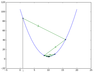
To reach the result of 9.99999773021 required 57 iterations.
12 13 14 15 16 17 18 19 20 21 22 23 24 25 26 27 28 29 30 31 32 33 34 35 36 | |
Hill descent without overshooting
The following algo is similar, but avoids overshooting: in case we overshoot, it keeps adjusting the step-size until we land on the left side of the minimum.
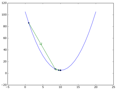
This time to get the result of 9.99999773022 required only 21 iterations, quite a bit better than above, but that of course may be due to the function and the choosen stepsize.
12 13 14 15 16 17 18 19 20 21 22 23 24 25 26 27 28 29 30 31 32 33 34 | |
The common functions for above code
Function and direction
5 6 7 8 9 10 | |
Plotting
5 6 7 8 9 10 | |
Mathematical approach
The above 2 solutions are the naive implementations, that perform fairly well. The mathematical way would be to calculate the next x as:

with step η typically chosen as 0.1.
During the ensuing iterations η can be kept constant or decreasing eg.

Choosing the stepsize is an art!
Gradient descent
Similarly to above, for gradient descent we update the coefficients by moving in the negative gradient direction (gradient is direction of increase). The increment in gradient descent is:
